Geospatial Indexes — Point vs Region
Deep Dive on Geospatial Index Architecture in MarkLogic
 Minimum Llamaverse Version: 2
MarkLogic's geospatial capabilities fall into two distinct index families: point indexes and region indexes. They sound similar, but they model fundamentally different things. A point index says "this document has a location." A region index says "this document represents an area." Using the wrong one for your data produces queries that either fail silently or return incorrect results.
This is one of those topics where everything feels fine right up until a map dashboard goes very, very wrong.
The other key source of confusion is coordinate ordering. MarkLogic's default coordinate system (wgs84) expects (latitude, longitude). GeoJSON — the most common coordinate encoding in modern APIs — specifies (longitude, latitude). Mixing these two orderings is a silent bug: the query runs, returns results, and those results are geographically wrong. A location in the west of Ireland becomes a point in equatorial Africa, and nothing complains.
Understanding these two distinctions — point vs region, and coordinate ordering — covers the vast majority of geospatial bugs encountered in production MarkLogic systems.
In practice, teams get the best outcomes when they treat geospatial index choice as an architectural decision made before ingestion, not a post-load tuning step.
Preflight Decisions
Before creating any geospatial index, answer these three questions explicitly:
- Is each document a location, an area, or both?
- Are source coordinates lat-first or lon-first?
- Which query type matters most: near/within, or overlap/containment between areas?
MarkLogic geospatial design is one of the places where architecture choices determine whether your query layer stays fast and correct for years, or becomes a stream of silent bugs and expensive reindex work.
Most production failures come from two root causes:
- Index-model mismatch: point indexes used for region questions, or region indexes used for point workloads.
- Coordinate-system mismatch: lat/lon assumptions mixed with GeoJSON lon/lat reality.
Both failures can return valid-looking results that are geographically wrong.
An additional failure mode appears at scale: teams optimise for a single query pattern, then layer new product requirements on top without evolving index topology. The result is often a brittle query layer where every change requires risky index rewiring.
A practical production posture is to model geospatial intent in three buckets from day one:
- User-facing proximity queries (near, within radius).
- Policy or rules queries (inside zone, outside boundary).
- Analytical spatial relationships (intersects, overlaps, coverage drift over time).
When these three buckets are explicitly mapped to indexes and query paths, geospatial behaviour stays understandable even as dataset size and query diversity grow.
This deep dive focuses on getting those two decisions correct with concrete llamaverse examples, operational rollout guidance, and practical troubleshooting patterns.
The examples in this article assume the llamaverse (v2.0+) is deployed. The llamaverse sample data is freely available from github.com/cleverllamas/llamaverse — see the llamaverse article for full setup instructions.
Why Geospatial Design Fails in Production
Teams often discover geospatial complexity too late because the first demo works:
- A single circle query over a small dataset returns plausible results.
- Source data grows and adds mixed coordinate formats.
- Region containment questions arrive later from product or analytics teams.
- Existing index choices become either incorrect or too expensive.
Treat geospatial index strategy as a first-class data-model decision, not a tuning step.
Llamaverse Geospatial Baseline
The llamaverse contains movement telemetry at:
/cleverllamas/llamaverse/content/llama-movement/llama_location_history.json
That document stores movement rows as GeoJSON-style coordinate pairs (lon, lat). Before designing indexes, profile what is actually in the dataset.
xquery version "1.0-ml";

let $uri := "/cleverllamas/llamaverse/content/llama-movement/llama_location_history.json"
let $records := fn:doc($uri)/*:envelope/*:instance/*:llama-movement
let $llama-ids := fn:distinct-values($records/*:llamaId/fn:string())
let $lons := for $r in $records return xs:double($r/*:coordinates[1]/fn:string())
let $lats := for $r in $records return xs:double($r/*:coordinates[2]/fn:string())
let $aaron-id := "0c8bdb0d-ac62-49b7-ac74-94dbba46efa5"
let $aaron-count := fn:count($records[*:llamaId = $aaron-id])
return (
  "movement-uri: " || $uri,
  "total movement rows: " || fn:count($records),
  "distinct llama IDs: " || fn:count($llama-ids),
  "aaron rows: " || $aaron-count,
  "lon min/max: " || fn:min($lons) || " / " || fn:max($lons),
  "lat min/max: " || fn:min($lats) || " / " || fn:max($lats)
)
movement-uri: /cleverllamas/llamaverse/content/llama-movement/llama_location_history.json
total movement rows: 3360
distinct llama IDs: 20
aaron rows: 168
lon min/max: -9.9234931 / 4.329025
lat min/max: 52.073568 / 53.5144999
This gives you concrete volume and spread information to drive index choices.
Geospatial Index Families (What They Actually Mean)
| Index family | Models | Best-fit questions | Typical risk if misused |
|---|---|---|---|
| Point indexes | Single location per logical record | Near, within radius, point-in-region filters | Cannot correctly answer area overlap/containment between boundaries |
| Region indexes | Spatial extent (polygon/line/box/circle) | Contains, intersects, overlaps, covers, covered-by | Higher cost for simple nearest/within point workloads |
A fast mental model:
- "Where is it?" usually means point index.
- "What area does it cover?" usually means region index.
- If you need both, configure both deliberately.
Query Cost Characteristics
Index selection is not just about correctness. It also determines how quickly you can answer the question under load.
| Query style | Typical geometry cost | Typical index fit |
|---|---|---|
| Point to circle / point to polygon filter | Low to medium | Point index |
| Region contains point | Medium | Region index (or point + region query, depending on source model) |
| Region overlaps region | High | Region index |
| Nearest N points | Low | Point index |
If your p95 response time degrades rapidly as polygon complexity increases, that is usually a sign that region semantics are being applied too broadly in paths that should remain point-first.
Recommended Index Pack for Llamaverse Workloads
| Data shape | Example source | Recommended index | Coordinate system | Why |
|---|---|---|---|---|
Point-like location docs (lat + lon) | Derived movement point documents, farm location docs | Geospatial JSON Property Pair Index (lat, lon) | wgs84 | Fast near/within queries and simple operational tuning |
GeoJSON-like [lon, lat] coordinate arrays | /cleverllamas/llamaverse/content/llama-movement/llama_location_history.json | Geospatial Path Index on coordinate path | wgs84/long-lat-point | Uses source ordering directly with no transform |
| Polygon boundaries | Grazing zones, farm boundaries, service territories | Geospatial Region Path Index on boundary path | wgs84/long-lat-point for GeoJSON | Required for contains/intersects/overlaps area logic |
| Mixed workloads (point + region) | Point telemetry + region geofences | Both point and region indexes | Match each source | Keeps near queries and containment queries both efficient |
The key design idea is to match each query family to the cheapest correct index, not force one index type to do all jobs.
Point Index Deep Dive
Point indexes are ideal when each document has one location and queries are mostly "near/within".
The examples below use a point-like farm model with lat/lon properties.
{
  "name": "Sunny Llama Ranch",
  "region": "Connaught",
  "lat": 53.7946,
  "lon": -9.0143
}
xquery version "1.0-ml";

(: Demonstrates point-in-circle logic equivalent to indexed geospatial query  :)
(: semantics, but using a compact in-memory sample to stay runnable in any    :)
(: environment.                                                                :)
let $farms := (
  <farm name="Sunny Llama Ranch" lat="53.7946" lon="-9.0143"/>,
  <farm name="Misty Valley Farm" lat="53.9500" lon="-8.6500"/>,
  <farm name="Northern Plains Farm" lat="54.6000" lon="-7.9000"/>
)
let $centre := cts:point(53.7500, -9.0500)
let $radius-miles := 20
for $farm in $farms
let $point := cts:point(
  xs:double($farm/@lat/fn:string()),
  xs:double($farm/@lon/fn:string())
)
let $miles := cts:distance($point, $centre)
where $miles le $radius-miles
return fn:string($farm/@name)
Sunny Llama Ranch
Use point indexes for:
- Search-result filtering by distance.
- Geofencing against circles/boxes/polygons.
- High-throughput telemetry lookups.
Avoid point-only modelling when business logic needs area-to-area relationships.
Rich Example: Two-Stage Geofence Query
A robust production pattern combines both index families:
- Use point logic to shortlist nearby candidates cheaply.
- Use region logic to confirm exact zone membership.
xquery version "1.0-ml";

import module namespace geo = "http://marklogic.com/geospatial"
  at "/MarkLogic/geospatial/geospatial.xqy";

(: Stage 1: point-style shortlist by distance.                               :)
(: Stage 2: region-style confirmation against grazing zone boundaries.       :)
let $query-point := cts:point(53.80, -9.00)
let $radius-miles := 20

let $farms := (
  <farm name="Sunny Llama Ranch" lat="53.7946" lon="-9.0143"/>,
  <farm name="Misty Valley Farm" lat="53.95" lon="-8.65"/>,
  <farm name="Northern Plains Farm" lat="54.60" lon="-7.90"/>
)

let $zones := (
  <zone name="West Grazing Zone" points="53.77,-9.10 53.77,-8.90 53.86,-8.90 53.86,-9.10 53.77,-9.10"/>,
  <zone name="North-East Grazing Zone" points="54.30,-8.30 54.30,-7.70 54.75,-7.70 54.75,-8.30 54.30,-8.30"/>
)

let $nearby :=
  for $farm in $farms
  let $pt := cts:point(xs:double($farm/@lat), xs:double($farm/@lon))
  let $dist := cts:distance($query-point, $pt)
  where $dist le $radius-miles
  return <candidate name="{fn:string($farm/@name)}" miles="{fn:round($dist * 100) div 100}"/>

let $containing-zones :=
  for $zone in $zones
  let $vertices :=
    for $pair in fn:tokenize(fn:string($zone/@points), "\s+")
    let $parts := fn:tokenize($pair, ",")
    return cts:point(xs:double($parts[1]), xs:double($parts[2]))
  let $polygon := cts:polygon($vertices)
  where geo:contains($polygon, $query-point)
  return fn:string($zone/@name)

return
  <result>
    <query-point lat="53.80" lon="-9.00"/>
    <nearby-farms>{ $nearby }</nearby-farms>
    <containing-zones>{ for $z in $containing-zones return <zone>{ $z }</zone> }</containing-zones>
  </result>
<result>
  <query-point lat="53.80" lon="-9.00"/>
  <nearby-farms>
    <candidate name="Sunny Llama Ranch" miles="0.69"/>
    <candidate name="Misty Valley Farm" miles="17.67"/>
  </nearby-farms>
  <containing-zones>
    <zone>West Grazing Zone</zone>
  </containing-zones>
</result>
This keeps latency predictable while preserving geometry correctness.
Region Index Deep Dive
Region indexes are for boundary logic: zone containment, overlap, and intersection semantics.
{
  "name": "Western Grazing Zone",
  "managed_by": "Connaught Llama Authority",
  "boundary": {
    "type": "Polygon",
    "coordinates": [[
      [-9.10, 53.75],
      [-8.90, 53.75],
      [-8.90, 53.85],
      [-9.10, 53.85],
      [-9.10, 53.75]
    ]]
  }
}
xquery version "1.0-ml";

import module namespace geo = "http://marklogic.com/geospatial"
  at "/MarkLogic/geospatial/geospatial.xqy";

(: Demonstrates region containment semantics with a representative boundary.   :)
let $western-zone := cts:polygon((
  cts:point(53.77, -9.10),
  cts:point(53.77, -8.90),
  cts:point(53.86, -8.90),
  cts:point(53.86, -9.10),
  cts:point(53.77, -9.10)
))
let $query-point := cts:point(53.80, -9.00)
return
  if (geo:contains($western-zone, $query-point))
  then "Western Grazing Zone"
  else "No containing zone"
Western Grazing Zone
Core region relationship operators:
| Operator | Meaning |
|---|---|
contains | Indexed region contains query geometry |
covered-by | Indexed region is fully covered by query geometry |
covers | Indexed region fully covers query geometry |
intersects | Indexed region shares any area with query geometry |
overlaps | Indexed region overlaps without full containment |
within | Indexed region lies entirely within query geometry |
Region indexes cost more than point indexes because polygon math is heavier. Use them where the question requires geometry semantics, not where distance-to-point logic is enough.
Rich Example: Operator Fixtures You Can Trust
When teams debate geospatial operators, ambiguity causes regressions. Keep a tiny fixture set with known expected outcomes.
xquery version "1.0-ml";

import module namespace geo = "http://marklogic.com/geospatial"
  at "/MarkLogic/geospatial/geospatial.xqy";

let $zone-a := cts:polygon((
  cts:point(53.70, -9.20),
  cts:point(53.70, -8.90),
  cts:point(53.92, -8.90),
  cts:point(53.92, -9.20),
  cts:point(53.70, -9.20)
))

let $zone-b := cts:polygon((
  cts:point(53.80, -9.05),
  cts:point(53.80, -8.70),
  cts:point(54.02, -8.70),
  cts:point(54.02, -9.05),
  cts:point(53.80, -9.05)
))

let $query-point := cts:point(53.84, -8.98)

let $a-contains-point := geo:contains($zone-a, $query-point)
let $b-contains-point := geo:contains($zone-b, $query-point)
let $zones-intersect := geo:intersects($zone-a, $zone-b)
let $a-contains-b := geo:contains($zone-a, $zone-b)
let $b-contains-a := geo:contains($zone-b, $zone-a)

return (
  fn:concat("A contains query point: ", $a-contains-point),
  fn:concat("B contains query point: ", $b-contains-point),
  fn:concat("A intersects B: ", $zones-intersect),
  fn:concat("A contains B: ", $a-contains-b),
  fn:concat("B contains A: ", $b-contains-a)
)
A contains query point: true
B contains query point: true
A intersects B: true
A contains B: false
B contains A: false
This gives you a deterministic correctness harness before rolling operator changes into production.
Coordinate Systems and the Silent GeoJSON Bug
MarkLogic default wgs84 expects (lat, lon). GeoJSON stores (lon, lat). Mixing these two is the single most common geospatial production bug.
xquery version "1.0-ml";

(: The coordinate ordering gotcha: wgs84 expects (lat, lon), but GeoJSON      :)
(: stores coordinates as [lon, lat].                                          :)
(:                                                                            :)
(: With wgs84 (lat-first), this point is in western Ireland:                 :)
let $correct := cts:point(53.7946, -9.0143)

(: With wgs84/long-lat-point (lon-first), the same numbers become a point    :)
(: in Russia — a completely different location.                               :)
let $wrong := cts:point(-9.0143, 53.7946)   (: This is (lat=-9, lon=53) :)

return (
  "lat-first (wgs84):        " || fn:string($correct),
  "lon-first (long-lat):     " || fn:string($wrong)
)
lat-first (wgs84):        53.7946,-9.0143
lon-first (long-lat):     -9.0143,53.7946
Now with live llamaverse movement coordinates:
xquery version "1.0-ml";

let $first :=
  fn:doc('/cleverllamas/llamaverse/content/llama-movement/llama_location_history.json')
  /*:envelope/*:instance/*:llama-movement[1]
let $lon := xs:double($first/*:coordinates[1]/fn:string())
let $lat := xs:double($first/*:coordinates[2]/fn:string())
let $centre := cts:point(53.5138, -9.9228)
let $correct := cts:point($lat, $lon)
let $swapped := cts:point($lon, $lat)
return (
  "source lon,lat: " || $lon || "," || $lat,
  "distance with correct order (miles): " || cts:distance($correct, $centre),
  "distance with swapped order (miles): " || cts:distance($swapped, $centre)
)
source lon,lat: -9.9234084,53.5137279
distance with correct order (miles): 0.0255778956432181
distance with swapped order (miles): 5720.9905072203
Swapping coordinate order turns a local movement point into a location thousands of miles away. No syntax error warns you.
Coordinate-system mapping:
| Stored ordering | Coordinate system |
|---|---|
| (lat, lon) | wgs84 |
| (lon, lat) GeoJSON | wgs84/long-lat-point |
| (lat, lon) with double precision | wgs84/double |
| (lon, lat) with double precision | wgs84/double/long-lat-point |
Operational guardrails that prevent this class of bug:
- Add ingestion-time assertions for coordinate ranges and ordering expectations.
- Keep one canary query in CI that checks a known point and known expected distance.
- Include coordinate-order metadata in source contracts so feed changes are not silent.
Llamaverse Movement Analysis Example
Before introducing indexes, this analytical pass validates spatial coherence for one tracked llama.
xquery version "1.0-ml";

let $uri := "/cleverllamas/llamaverse/content/llama-movement/llama_location_history.json"
let $records :=
  fn:doc($uri)/*:envelope/*:instance/*:llama-movement[*:llamaId = "0c8bdb0d-ac62-49b7-ac74-94dbba46efa5"]
let $centre := cts:point(53.5138, -9.9228)
let $hits :=
  for $r in $records
  let $lon := xs:double($r/*:coordinates[1]/fn:string())
  let $lat := xs:double($r/*:coordinates[2]/fn:string())
  let $point := cts:point($lat, $lon)
  let $miles := cts:distance($point, $centre)
  where $miles le 0.25
  return $miles
return (
  "aaron total rows: " || fn:count($records),
  "rows within 0.25 miles of centre: " || fn:count($hits),
  "closest miles: " || fn:min($hits),
  "furthest miles within window: " || fn:max($hits)
)
aaron total rows: 168
rows within 0.25 miles of centre: 168
closest miles: 0.00395853094506708
furthest miles within window: 0.0637264530896653
This kind of profile helps choose sensible geofence radius values and detect outlier points early.
Visual Query Walkthroughs
Spatial bugs are often easier to detect visually than by reading query text alone. Two lightweight graphics usually provide the highest value:
- Point-versus-region query flow diagram for architecture conversations.
- Coordinate-order impact diagram for onboarding and incident reviews.
- Region operator fixture map for query correctness discussions.
- Rollout workflow diagram for delivery and operations planning.
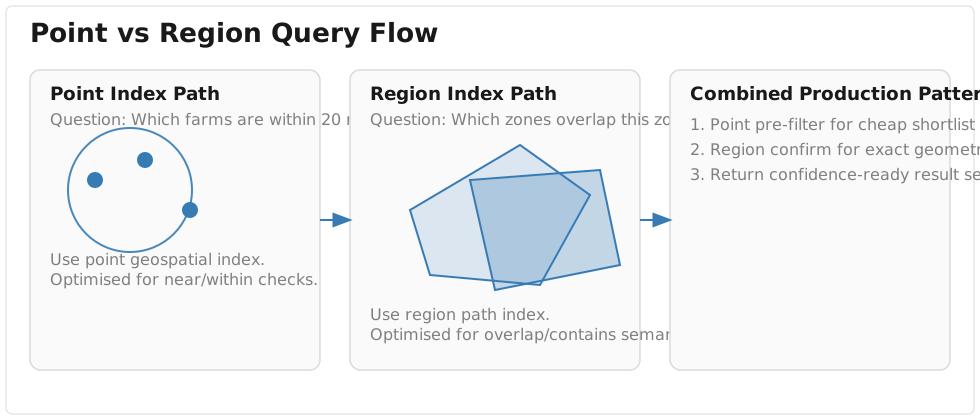
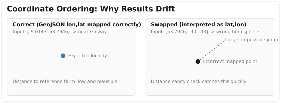
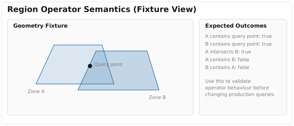
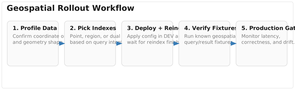
For production environments, pair each graphic with one runnable query and one expected result file. That keeps diagrams tied to executable truth rather than becoming static documentation drift.
End-to-End Design Decision Matrix
| Query intent | Correct index strategy | Coordinate guidance |
|---|---|---|
| Find llama events near a point | Point index (pair or path geospatial point) | Use source ordering consistently |
| Find farms inside a polygon | Point index + polygon region filter | Match index coordinate system to source order |
| Find which zones cover this event | Region index on zone boundary | GeoJSON zones usually need wgs84/long-lat-point |
| Find overlapping service territories | Region index | Validate overlap semantics with known fixtures |
| Mix telemetry + geofences | Both point and region indexes | Keep both pipelines explicit |
Design Checklist Before Production Deployment
- Do all coordinate sources have explicit ordering documentation?
- Is each query path mapped to a known index family?
- Do you have fixture-based operator tests for region semantics?
- Is there one visual artefact that makes the query path obvious to non-specialists?
- Can on-call engineers run one fast sanity query during incidents?
Configuration and Rollout Strategy
Geospatial indexes are configured through Admin UI or the Admin XQuery module. The Management REST API does not configure geospatial indexes directly.
Admin UI paths:
| Index type | Admin UI path |
|---|---|
| Geospatial JSON Property Pair | Admin -> Databases -> db -> Geospatial JSON Property Pair Indexes |
| Geospatial Region Path | Admin -> Databases -> db -> Geospatial Region Path Indexes |
| Geospatial Path Indexes | Admin -> Databases -> db -> Geospatial Path Indexes |
| Geospatial Element Pair | Admin -> Databases -> db -> Geospatial Element Pair Indexes |
Rollout guidance:
- Add indexes in low-traffic windows.
- Monitor reindex completion before benchmarking.
- Validate with known-good fixtures before releasing query features.
- Document coordinate assumptions next to ingestion logic.
Performance Deep Dive
| Workload | Typical winner | Why |
|---|---|---|
| High-volume near queries | Point index | Cheaper geometry checks |
| Region containment/overlap analytics | Region index | Correct geometry semantics |
| Mixed dashboard + boundary checks | Dual index strategy | Avoids overloading one index family |
Performance anti-patterns:
- Running region overlap logic against centroid points.
- Overusing region indexes for simple nearest-point lookups.
- Deferring coordinate-system validation until after production rollout.
Practical benchmarking pattern:
- Benchmark point-only path with fixed radius and growing candidate count.
- Benchmark region-only path with growing polygon complexity.
- Benchmark combined two-stage path and track shortlist size sensitivity.
This usually reveals that combined paths produce the best correctness-to-latency ratio for mixed workloads.
Troubleshooting Matrix
| Symptom | Likely cause | Fast check | Fix |
|---|---|---|---|
| Empty results for known nearby points | Coordinate-system mismatch | Compare one known point with both orderings | Switch to wgs84/long-lat-point for GeoJSON |
| Results in wrong geography | Swapped lon/lat | Run a distance sanity query against known centre | Correct ingestion transform or index config |
| Region query errors about missing index | Region path index absent | Check database index config | Add required region index and reindex |
| Point queries slow under load | Region index used for point-only workload | Review query/index pairing | Add point index and route query accordingly |
| Correctness drifts after data feed change | Upstream coordinate format changed | Profile incoming sample payloads | Version and validate ingestion mapping |
Incident Triage Sequence
When geospatial incidents occur, use this order:
- Validate coordinate ordering on one known record.
- Validate index presence and coordinate-system settings.
- Re-run fixture queries with known expected answers.
- Compare point-only and region-only paths to isolate the failing stage.
Final Takeaways
High-quality MarkLogic geospatial systems come from three explicit decisions:
- Pick the correct index family for the question (point vs region).
- Lock coordinate-ordering assumptions early and enforce them at ingestion.
- Validate with real dataset fixtures (like llamaverse movement history) before deploying to production.
Get these right and geospatial search becomes a reliable strength, not an intermittent production incident source.
Get them wrong and your incident channel learns far more about coordinate systems than anyone wanted.
Need Some Help?
Looking for more information on this subject or any other topic related to MarkLogic? Contact Us (info@cleverllamas.com) to find out how we can assist you with consulting or training!
Scope Note: Reverse Geospatial Queries
This article focuses on forward geospatial queries — finding points within a region or regions containing a point. Reverse geospatial queries (also called "inverse" or "containment queries") are implemented at varying levels of completeness across MarkLogic versions and depend heavily on your spatial data structures and use cases.
If you need to run reverse geospatial queries, evaluate them carefully with your MarkLogic version and dataset before committing to production. Different approaches work best for different query patterns and data distributions.
Working with Reverse Geospatial Queries
If you're evaluating reverse geospatial approaches or running into unexpected behaviour with containment queries, reach out to us at info@cleverllamas.com — we can help you architect a solution tailored to your data and query patterns.
- Preflight Decisions
- Why Geospatial Design Fails in Production
- Llamaverse Geospatial Baseline
- Geospatial Index Families (What They Actually Mean)
- Query Cost Characteristics
- Recommended Index Pack for Llamaverse Workloads
- Point Index Deep Dive
- Rich Example: Two-Stage Geofence Query
- Region Index Deep Dive
- Rich Example: Operator Fixtures You Can Trust
- Coordinate Systems and the Silent GeoJSON Bug
- Llamaverse Movement Analysis Example
- Visual Query Walkthroughs
- End-to-End Design Decision Matrix
- Design Checklist Before Production Deployment
- Configuration and Rollout Strategy
- Performance Deep Dive
- Troubleshooting Matrix
- Incident Triage Sequence
- Final Takeaways
- Scope Note: Reverse Geospatial Queries